
SEL threshold estimates from limited test data
Enter one heavy-ion observation (latchups at a test LET, a measured cross section, a saturated cross section, or a run with no latchup) and the device class. You get the threshold LET at σ = 10⁻⁸ cm² with confidence bounds or, after a null, how likely the part is to be susceptible at all.
Test observation
Device
Why the conventions behind this tool are what they are: the 1e7 test fluence, 3.7 versus 2.3 for a null result, LET 15, 37, 60 and 75, why latchup is tested hot, why range matters for latchup.
Predicted SEL threshold (LET at σ = 10⁻⁸ cm²)
How the answer was reached
Cross-checks and population context
How it works
From one test result to a threshold with bounds
Start from one observation
Latchups at a test LET, a measured cross section, a saturated cross section, or a run with no latchup at all, with the fluence and whether the part was tested hot.
Place it on the historical trend
Parts that latch at low LET tend to have large cross sections. The tool reads that trend, fitted to thousands of historical SEL results, at your test LET and for your device class and era.
Read the threshold and its bounds
Monte Carlo draws around the trend give the median and the confidence interval, and a part that latched at the test LET must have its threshold below it. After a null, the tool updates the chance that the part is susceptible at all.
About this tool what the numbers come from
Single-event latchup threshold LET (at σ = 10⁻⁸ cm²) with confidence bounds, inferred from a cross-section measurement at any test LET, from a saturated cross section, or from a null result. Every number comes from the Extended Historical SEL Priors (EHSP), release 2026-09: Ladbury's historical-data SEL priors (IEEE TNS 2024, 2025) rebuilt on a mechanism-screened, uniformly refit corpus of 4,610 SEL part-entries, with an errors-in-variables onset trend, class and era conditioning, iso-LET predictors and censoring-aware susceptibility priors. The methodology section below documents every step with figures.
Methodology: the Extended Historical SEL Priors behind this tool 18 sections, figures and tables
Methodology: the Extended Historical SEL Priors (EHSP) behind this tool
Everything this page computes comes from one machine-readable model file, ehsp-2026-09.js (Extended Historical SEL Priors, release 2026-09, built 2026-09-02). The name is deliberate: Ladbury's papers [1], [3], [6] built "historical-data-driven prior probability distributions" for SEL from archives of test data, and this model extends that construction, keeping its form (a lognormal onset versus cross-section prior and per-technology susceptibility probabilities) while rebuilding both from a much larger, uniformly refit corpus. This section documents how the file was built: the corpus, the extraction and fitting, the uniform definitions of onset and saturation, the errors-in-variables trend model and its ladder of ingredients, class, process and era conditioning with partial pooling, the SRAM special case, the iso-LET predictors used for non-saturated measurements, the temperature factors, the mechanism screen, the censoring-aware susceptibility priors and their validation, and finally how each input mode of the tool uses the model. Published sources are cited; proprietary test reports and campaign records contributed to the fits and are identified only as proprietary. Numbers in this section are read from the model file and its companion tables at build time, so they cannot drift from what the tool computes.
1. Overview and provenance
Ladbury showed in [1] and [2] that a large database of SEL-susceptible parts supports two practical priors for parts with little or no heavy-ion data: a power law between onset LET and limiting cross section, usable as a Bayesian prior for under-constrained Weibull fits, and technology-level probabilities of susceptibility. Both inherit the heterogeneity of their inputs: Weibull parameters fit by many authors under differing conventions, and expert point estimates for susceptibility. EHSP rebuilds both from primary per-run data under one reproducible pipeline, and adds four things the original framework lacked: a uniform saturation definition, a predictor that works from a single non-saturated measurement, an explicit mechanism screen, and censoring-aware prior updates that use immune parts as evidence.
The model is versioned and shipped as a single JSON file with reference implementations in Python and JavaScript that pass the same 14 embedded test vectors. The public copy on this site is byte-for-byte the internal model with two changes: stratum names and free-text provenance fields that named proprietary sources were rewritten, and a numeric digest of every value was checked before and after that rewrite. The definitions the model file states, and which every consumer of it must state, are: onset is the LET at which the Poisson-MLE Weibull fit to per-run data crosses σ = 10⁻⁸ cm²; saturation is σ(80), the fitted cross section at LET 80 MeV·cm²/mg; susceptible means onset at or below 75 MeV·cm²/mg at hot-equivalent conditions, with room-temperature null tests mapped by a factor 0.74 in LET; and era splits parts tested or published before 2010 (legacy) from 2010 and later (modern).
2. Data sources and extraction
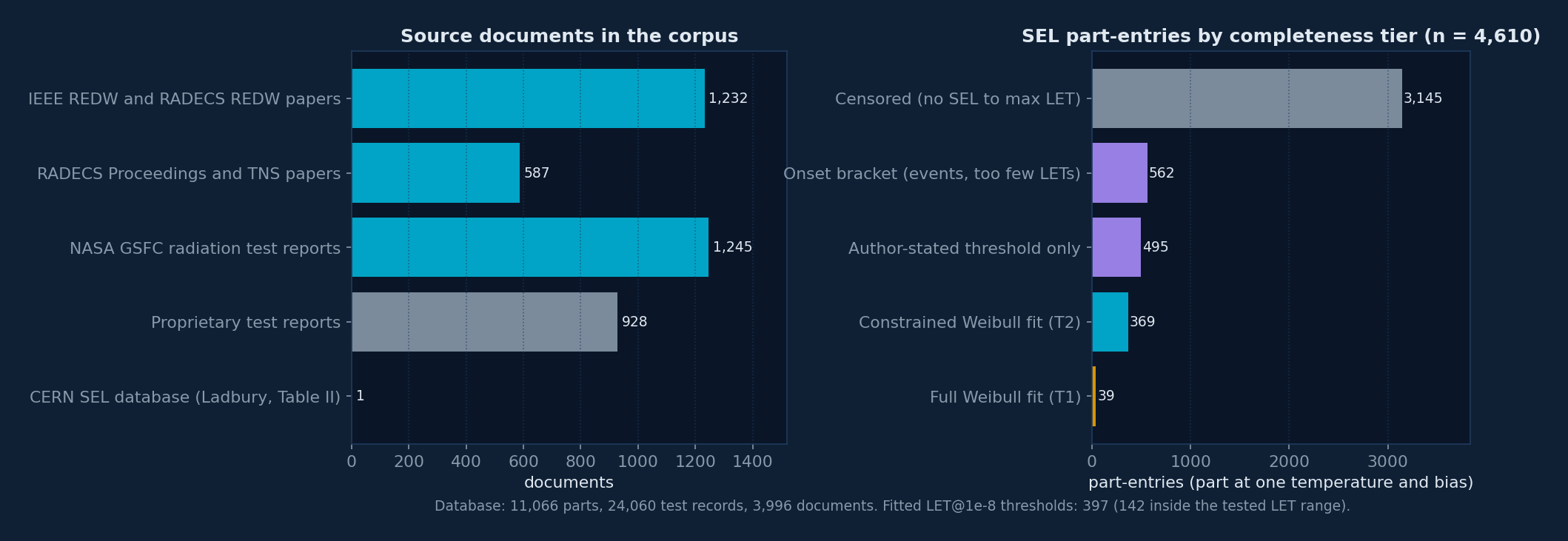
The corpus (Table 1) assembles the complete IEEE Radiation Effects Data Workshop record and the RADECS data-workshop record from 1992 to 2025, the RADECS Proceedings and IEEE Transactions on Nuclear Science literature from 1991 to 2025 screened for SEL data papers, the NASA Goddard radiation test reports and summaries, proprietary heavy-ion test reports and structured campaign logs, and the CERN SEL database of Coronetti and García Alía as published in Table II of [2]. Public and proprietary parts are pooled for every fit; the figures in this section plot public entries with their source type and proprietary entries as anonymous points.
Table 1. Source documents
| Source | Documents | Notes |
|---|---|---|
| IEEE REDW and RADECS data-workshop papers, 1992 to 2025 | 1,232 | public; per-run tables re-extracted; figure-only results digitized |
| RADECS Proceedings and IEEE TNS papers, 1991 to 2025 | 587 | public; keyword-screened data papers, curve-extracted and digitized |
| NASA GSFC radiation test reports and summaries | 1,245 | public; threshold-level records, onset brackets and censored entries |
| Proprietary test reports and campaign records | 928 | proprietary; per-run tables; used in aggregate only, never shown individually |
| CERN SEL database, Table II of Ladbury [2] | 1 | public; all-susceptible sample; admitted to the onset CDF and used as an external check only |
Extraction was performed by supervised language-model agents working from written specifications with guard rules developed adversarially: two-column interleave misattribution, inverted immunity statements, misuse of the destructive flag, invented digits and unit conversions were the failure modes the rules target, and a verification pass over 464 papers produced roughly 600 corrections before any analysis. Zero-event runs with a stated fluence were captured as data, not discarded. Results reported only as figures were digitized under a separate specification (pixel calibration against gridlines, marker-only reading, explicit upper-limit flags, cross-checks against values stated in the text) with a quality grade per figure; points digitized from figures whose horizontal axis is proton energy rather than LET were kept but excluded from all LET fits. Cross-database adjudication against a commercial aggregate database, a component-catalog service and the CERN table detected systematic errors in both directions, and the process technology of every part carries a provenance and a confidence level.
The unit of analysis is the part-entry: one part at one temperature and one bias condition. Every part-entry receives a completeness tier (Table 2). A null run at fluence F demonstrates only that σ is below 2.3 / F at 95% confidence; a 10⁷ ions/cm² run therefore proves σ < 2.3 × 10⁻⁷ cm², which is not immunity at the 10⁻⁸ level, and the prior-update likelihood of Section 13 encodes exactly that.
Table 2. Completeness tiers (4,610 part-entries)
| Tier | Part-entries | What it carries |
|---|---|---|
| T0, censored: no SEL up to the maximum clean LET | 3,145 | carries the demonstrated bound 2.3 / fluence at that LET |
| T3, onset bracket: events observed but too few LETs for a fit | 562 | onset bounded between the highest clean and lowest latching LET |
| T3, author-stated threshold only (no run table) | 495 | salvaged as an onset bracket or a censor level |
| T2, constrained Weibull fit | 369 | fit with at least one parameter at a bound or few points |
| T1, full Weibull fit | 39 | all four parameters determined |
3. Fitting and uniform definitions
Poisson maximum-likelihood Weibull fits
Each part-entry with per-run data is fit with the four-parameter Weibull σ(L) = σsat [1 − exp(−((L − L0)/W)s)] by Poisson maximum likelihood: a run with N events at fluence F and LET L contributes Poisson(N; σ(L)·F), so zero-event runs enter the likelihood as data. Digitized upper-limit markers are converted to zero-event runs at the implied fluence 2.3/σlimit, and cross-section-only points (digitized figures without fluence) enter as down-weighted lognormal pseudo-likelihoods (0.3 dex, weight 0.5). The optimizer is a bounded multi-start Nelder-Mead; the likelihood is the same family as the generalized linear model fitter of [1]. Fits with runaway width (W ≥ 500) or shape below 0.6 are flagged degenerate and excluded from all trend work. Fit parameters are stored at full precision: an earlier build rounded saturation values below 5 × 10⁻⁶ cm² to zero and silently removed small-σ parts from the trend, a defect the sanity battery of Section 10 caught.
Uniform onset: LET at σ = 10⁻⁸ cm²
Author-reported thresholds conflate the Weibull onset parameter L0, the lowest LET with events, and the highest LET without. Onset is instead defined as the LET at which the fitted curve crosses 10⁻⁸ cm², with a bracketing flag: measured if the crossing lies inside the tested LET range, extrapolated otherwise. The definition is insensitive to the level (the median shift between 10⁻⁷ and 10⁻⁹ definitions is 1 MeV·cm²/mg) but the flag matters: 64% of the 10⁻⁸ crossings in the current fit set lie below the lowest tested LET, and 18% of fits pin L0 at zero. This is why the errors-in-variables model of Section 6 treats extrapolated thresholds as intervals rather than as values, and why, for conservative use, extrapolated thresholds should be floored at the lowest tested LET.
Uniform saturation: σ(80)
Quoting the cross section at the highest tested LET understates saturation for any part not tested to its plateau and drags such parts leftward on the trend. Saturation is therefore defined as the fitted cross section at a reference LET of 80 MeV·cm²/mg, flagged measured-range when the tested range reaches at least 72 and fit-extrapolated otherwise. On measured-range parts the ratio σ(80)/σ(Lmax) has median 0.97 with 79% within a factor of two (n = 89); the residual spread is fit uncertainty at the plateau, not bias. On the σ(80) axis the corpus trend becomes coincident with the CERN fit of [2], and the earlier 20% prefactor gap between the two, reported in an internal comparison memo, turned out to be a saturation-definition artifact. The measured-range subset alone gives LET0 = 1.165 σ(80)-0.2604 (R² = 0.552, sln = 0.801, n = 87): steeper and tighter, because it excludes the parts whose fitted plateau is itself uncertain.
4. The onset versus saturation trend and the CERN cross-check
Figure 2 plots onset against σ(80) for the 303 fitted part-entries that survive the degenerate-fit and mechanism screens (176 public, 127 proprietary; 192 with extrapolated thresholds drawn as intervals). Ordinary least squares on the point estimates gives LET0 = 2.262 σ(80)-0.166 with R² = 0.326 and lognormal scatter sln = 0.936. The CERN trend of [2], LET0 = 1.9638 σ-0.192 with sln = 0.82 on 51 curated parts, is drawn for comparison: with a fully independent corpus, a different extraction pipeline and a different threshold definition, the exponents agree within the bootstrap uncertainty of Section 5 and the two lines are visually indistinguishable over five decades of σ. That is strong evidence the power law is device physics, onset and sensitive area scaling together, rather than an artifact of the CERN sample.
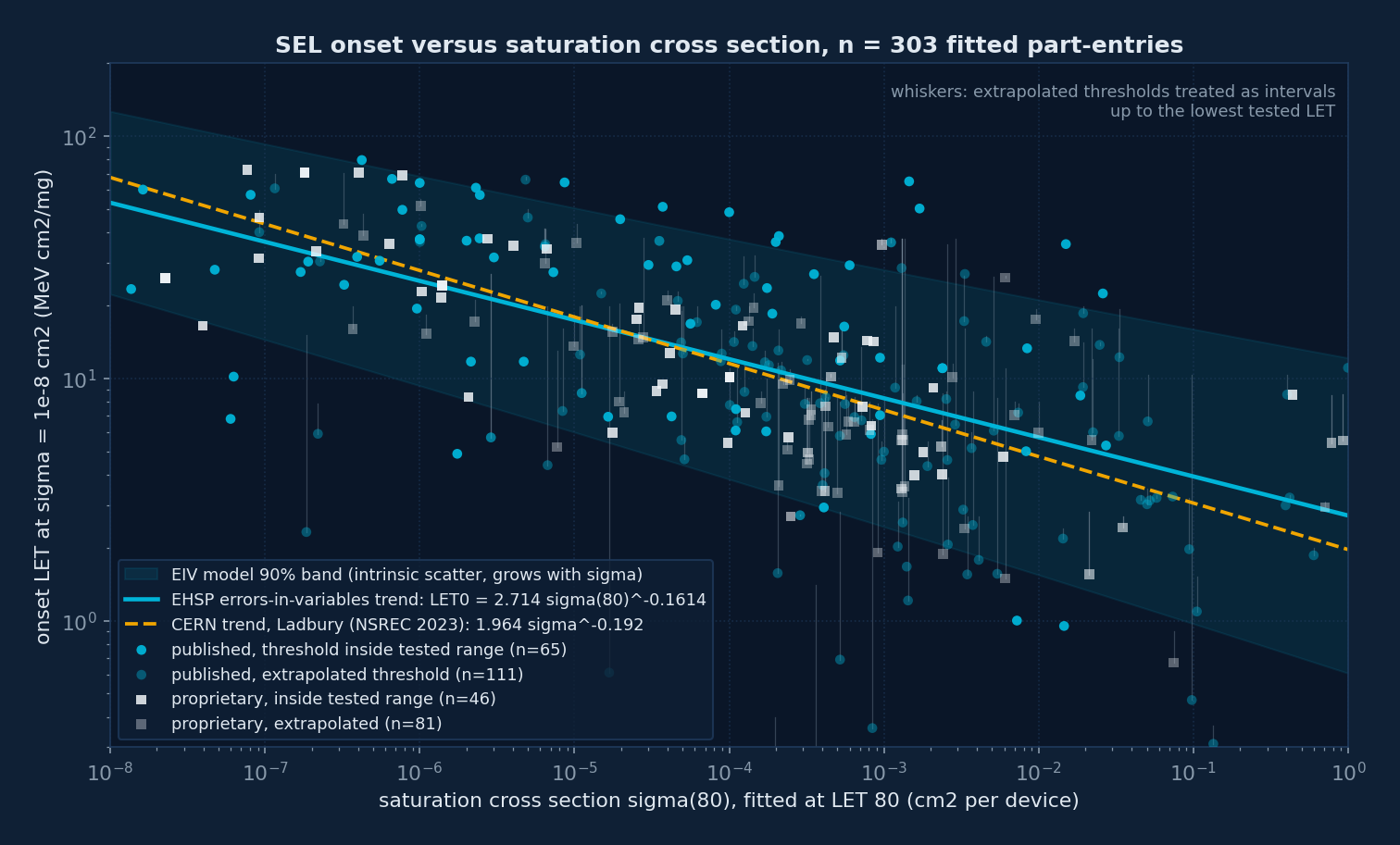
The scatter is heteroscedastic (Table 3): the residual standard deviation about the full model is 0.7 to 0.9 in natural log units for σ(80) between 10⁻⁸ and 10⁻⁴ cm² and 1.0 to 1.1 above 10⁻⁴, and the extreme decade (0.1 to 1 cm², whole-die SRAM and large or multi-die devices) sits well above the line. A constant-sln lognormal is therefore an approximation that is conservative at moderate σ and optimistic at extreme σ; the full model lets intrinsic scatter grow with σ.
Table 3. Residual scatter about the full model by decade of σ(80)
| σ(80) decade (cm²) | n | residual sd (ln units) |
|---|---|---|
| 10-8 to 10-7 | 13 | 0.718 |
| 10-7 to 10-6 | 22 | 0.881 |
| 10-6 to 10-5 | 38 | 0.801 |
| 10-5 to 10-4 | 41 | 0.802 |
| 10-4 to 10-3 | 94 | 0.990 |
| 10-3 to 10-2 | 55 | 0.973 |
| 10-2 to 10-1 | 27 | 1.022 |
| 10-1 to 100 | 13 | 1.068 |
5. Per-part uncertainty and bootstrap
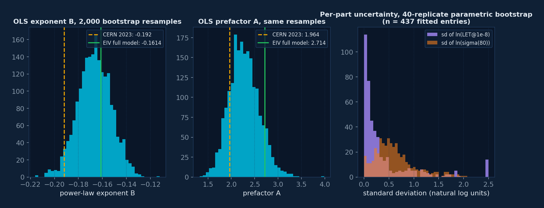
Two kinds of uncertainty are quantified. The uncertainty of the trend itself comes from a nonparametric bootstrap of the OLS fit (2,000 resamples of part-entries): exponent -0.1665 with 90% interval [-0.1898, -0.1433] and prefactor 2.257 [1.789, 2.81]. The CERN values (-0.192, 1.9638) lie inside or at the edge of these intervals. Collapsing to one worst-case entry per part leaves the exponent unchanged and widens the scatter, so duplicated temperature and bias entries do not drive the result.
The uncertainty of each part's coordinates comes from a 40-replicate parametric bootstrap of its Poisson Weibull fit: synthetic run tables are drawn from the fitted curve at the real fluences, refit, and the standard deviations of ln LET0 and ln σ(80) across replicates are recorded (medians 0.161 and 0.529 natural-log units over 437 fitted entries). Sibling entries that share a run table inherit their group value. These per-part uncertainties are the measurement-error terms of the errors-in-variables model.
6. The errors-in-variables model and its ladder
Ordinary least squares on point estimates ignores three things: both axes are fitted quantities with uncertainty, extrapolated thresholds are one-sided statements rather than values, and the scatter is visibly σ-dependent. The model fit by maximum likelihood is
τi² = s(xi)² + sy,i² + b²·sx,i², ln s(x) = c0 + c1·(x − x̄)
measured thresholds: Normal(yi | a + b xi + c hoti, τi)
extrapolated thresholds: interval-censored on [ln Lc − sy,i, ln Lmin,tested]
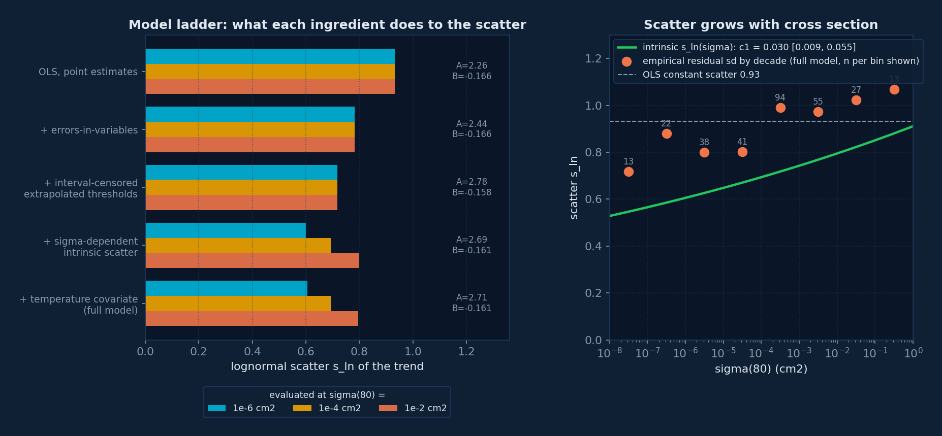
where sy,i and sx,i are the per-part bootstrap uncertainties of Section 5, Lc is the fitted 10⁻⁸ crossing and Lmin,tested is the lowest LET at which the part was tested. The fitted values are A = ea = 2.714, B = -0.1614 (90% interval [-0.182, -0.139]), c0 = -0.3511, c1 = 0.0296 (90% interval [0.009, 0.055]), x̄ = -8.7165, on n = 303 entries of which 192 are interval-censored. The intrinsic scatter runs from sln = 0.605 at σ(80) = 10⁻⁶ cm² to 0.795 at 10⁻² cm². The temperature coefficient is null (c = -0.045, interval spanning zero) for the physical reason given in Section 11.
Table 4 and Figure 4 show what each ingredient does. Accounting for measurement error removes noise from the scatter estimate (0.932 to 0.782); interval-censoring raises the prefactor, because true onsets lie above the extrapolated crossings; the σ-dependent scatter term is significant; and the temperature covariate changes nothing. This is the reference relation the tool uses whenever no class trend applies.
Table 4. Model ladder
| Model | A | B | chot | sln at 10⁻⁶ | at 10⁻⁴ | at 10⁻² |
|---|---|---|---|---|---|---|
| OLS (point estimates, constant scatter) | 2.262 | -0.1660 | 0.932 | 0.932 | 0.932 | |
| + errors-in-variables | 2.435 | -0.1660 | 0.782 | 0.782 | 0.782 | |
| + interval-censored extrapolated thresholds | 2.776 | -0.1575 | 0.718 | 0.718 | 0.718 | |
| + sigma-dependent intrinsic scatter | 2.695 | -0.1611 | 0.601 | 0.693 | 0.799 | |
| + temperature covariate (full model) | 2.714 | -0.1614 | -0.045 | 0.605 | 0.694 | 0.795 |
7. Class and process conditioning with partial pooling
Device class (converter, processor, power, logic, FPGA, memory, amplifier) and process family (bulk CMOS, BiCMOS, BCD and smart power) are known for most parts and shift the trend. Fitting every class separately would overfit the small ones, so class-by-era slopes and intercepts are partially pooled toward the global fit with DerSimonian-Laird shrinkage [7]: each group's OLS estimate is pulled toward the global value by a weight that depends on its own standard error and the between-group spread estimated from the data. The between-class spread of slopes is small (τB = 0.054) and the spread of intercepts is large (τlnA = 0.68): slopes are nearly common across classes, intercepts are not, so class conditioning acts mainly through the intercept. Converters and logic sit low on the trend, power and bulk CMOS sit high. Groups with fewer than eight entries fall back to the global errors-in-variables trend, and the tool flags when that happens.
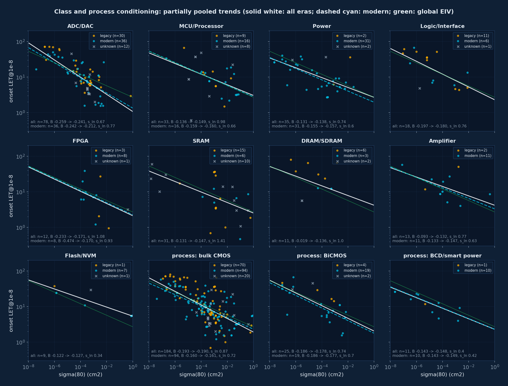
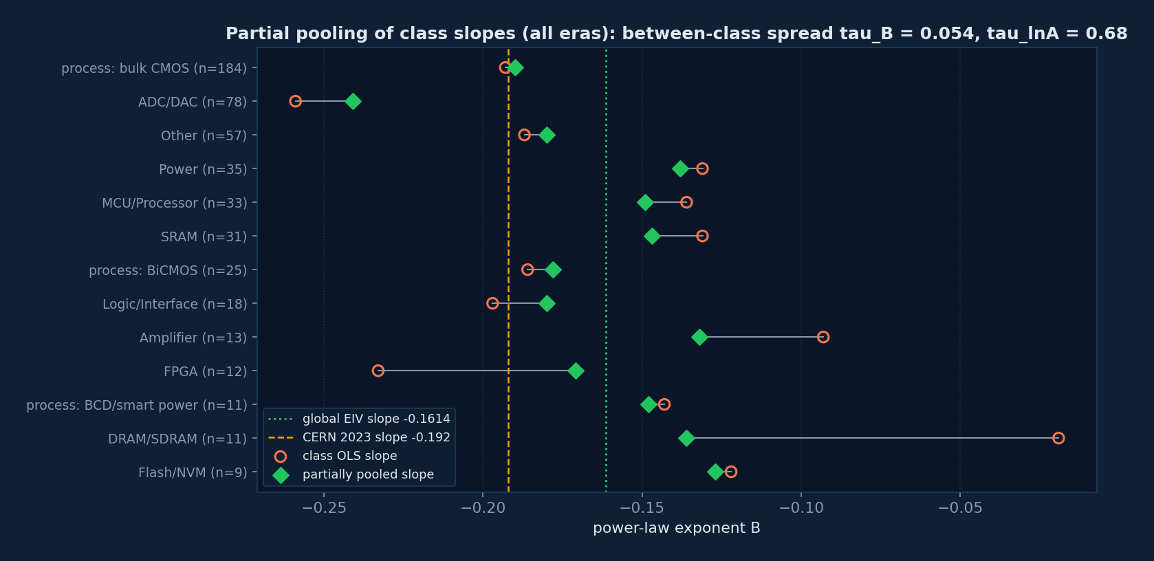
Table 5. Partially pooled class trends, modern era (used by the saturated-cross-section mode by default)
| Group | n | A (OLS) | A (pooled) | B (OLS) | B (pooled) | shrinkage of B | sln |
|---|---|---|---|---|---|---|---|
| process: bulk CMOS | 94 | 2.31 | 2.33 | -0.160 | -0.161 | 0.12 | 0.72 |
| ADC/DAC | 36 | 1.05 | 1.35 | -0.242 | -0.212 | 0.38 | 0.77 |
| Power | 31 | 1.85 | 1.97 | -0.155 | -0.157 | 0.20 | 0.60 |
| process: BiCMOS | 19 | 1.53 | 1.79 | -0.186 | -0.177 | 0.36 | 0.70 |
| MCU/Processor | 16 | 2.83 | 2.80 | -0.159 | -0.160 | 0.46 | 0.66 |
| Amplifier | 11 | 3.76 | 3.33 | -0.133 | -0.147 | 0.51 | 0.63 |
| process: BCD/smart power | 10 | 2.18 | 2.32 | -0.143 | -0.149 | 0.29 | 0.42 |
| FPGA | 8 | 0.19 | 2.28 | -0.474 | -0.170 | 0.97 | 0.93 |
Table 6. Partially pooled class trends, all eras
| Group | n | A (OLS) | A (pooled) | B (OLS) | B (pooled) | shrinkage of B | sln |
|---|---|---|---|---|---|---|---|
| process: bulk CMOS | 184 | 1.89 | 1.93 | -0.193 | -0.190 | 0.10 | 0.87 |
| ADC/DAC | 78 | 0.96 | 1.08 | -0.259 | -0.241 | 0.18 | 0.67 |
| Power | 35 | 2.71 | 2.71 | -0.131 | -0.138 | 0.25 | 0.74 |
| MCU/Processor | 33 | 3.20 | 3.06 | -0.136 | -0.149 | 0.50 | 0.98 |
| SRAM | 31 | 2.48 | 2.55 | -0.131 | -0.147 | 0.51 | 1.41 |
| process: BiCMOS | 25 | 1.86 | 2.06 | -0.186 | -0.178 | 0.33 | 0.74 |
| Logic/Interface | 18 | 2.05 | 2.31 | -0.197 | -0.180 | 0.47 | 0.76 |
| Amplifier | 13 | 5.89 | 4.20 | -0.093 | -0.132 | 0.57 | 0.77 |
| FPGA | 12 | 1.31 | 2.14 | -0.233 | -0.171 | 0.87 | 1.08 |
| process: BCD/smart power | 11 | 2.16 | 2.30 | -0.143 | -0.148 | 0.27 | 0.40 |
| DRAM/SDRAM | 11 | 17.90 | 4.21 | -0.019 | -0.136 | 0.82 | 1.00 |
| Flash/NVM | 9 | 5.62 | 5.39 | -0.122 | -0.127 | 0.12 | 0.34 |
The shrinkage column is the fraction of the distance from the OLS slope to the global slope that pooling removes; a value near one means the class contributes almost no slope information of its own. The scatter column is the OLS residual scatter of the group and is what the tool uses as sln for a class trend.
8. Era dependence
Era dependence is class-specific rather than universal (Figure 7, Table 7). Converters show a striking loss of correlation in modern parts (legacy R² = 0.76, sln = 0.48; modern R² = 0.50, sln = 0.77), consistent with heterogeneous latchup mitigation across modern converter processes. Bulk CMOS moves the other way (legacy sln = 1.01, modern 0.72), and processors are stable. The pooled mean onset declines only mildly with process generation. An earlier conclusion that modern trends are uniformly diffuse was partly an artifact of the highest-tested-LET saturation convention and of process-label pollution; it does not survive the uniform definitions. The tool therefore offers the era as an explicit choice for the saturation trend, with modern as the default, and uses the era only where a class has enough modern entries to support its own trend.
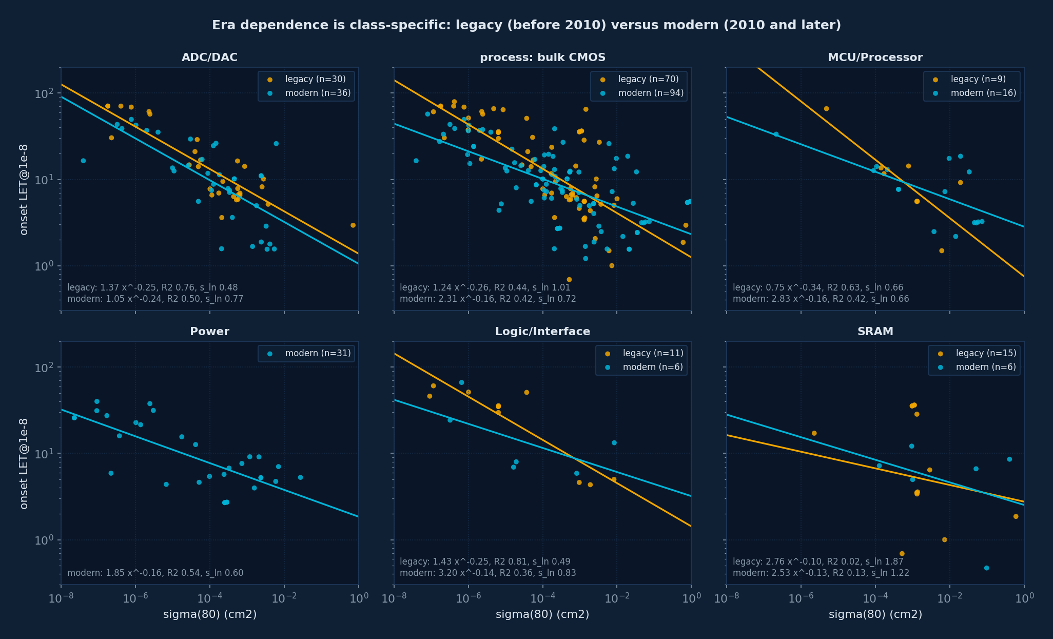
Table 7. Per-era OLS trends by class
| Group | Era | n | A | B | R² | sln |
|---|---|---|---|---|---|---|
| ADC/DAC | legacy | 30 | 1.38 | -0.245 | 0.76 | 0.48 |
| ADC/DAC | modern | 36 | 1.05 | -0.242 | 0.50 | 0.77 |
| Logic/Interface | legacy | 11 | 1.43 | -0.251 | 0.81 | 0.49 |
| Logic/Interface | modern | 6 | 3.20 | -0.140 | 0.36 | 0.83 |
| MCU/Processor | legacy | 9 | 0.75 | -0.338 | 0.63 | 0.66 |
| MCU/Processor | modern | 16 | 2.83 | -0.159 | 0.42 | 0.66 |
| Power | modern | 31 | 1.85 | -0.155 | 0.54 | 0.60 |
| SRAM | legacy | 15 | 2.76 | -0.096 | 0.02 | 1.87 |
| SRAM | modern | 6 | 2.53 | -0.131 | 0.13 | 1.22 |
| process: bulk CMOS | legacy | 70 | 1.25 | -0.257 | 0.44 | 1.01 |
| process: bulk CMOS | modern | 94 | 2.31 | -0.160 | 0.42 | 0.72 |
9. The SRAM special case
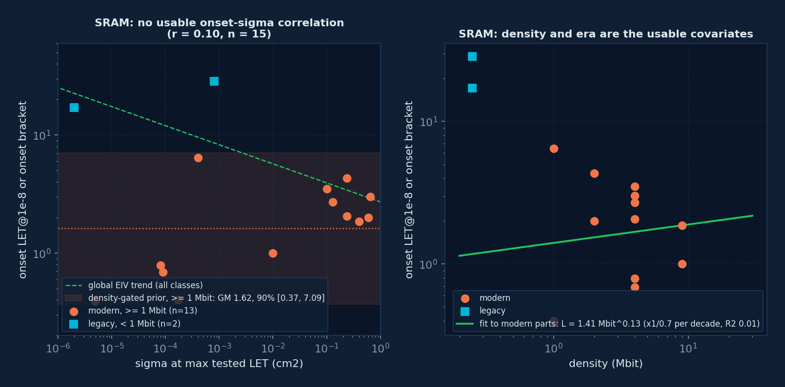
For SRAMs the onset versus saturation correlation vanishes: r = 0.10 over 15 vetted parts whose cross section is a whole-device latchup cross section rather than a per-bit upset figure. The population is two-component: legacy low-density devices (below 1 Mbit, n = 2, a thin sample) with geometric-mean onset 22.1, and modern high-density COTS devices (1 Mbit and above, n = 13) with geometric mean 1.62, sln = 0.9 and 90% interval [0.37, 7.09] MeV·cm²/mg. Across all 15 parts onset falls by about a factor 3.3 per decade of density (R² = 0.15), but that relation is carried by the legacy low-density parts; within the modern group density explains nothing (Figure 8, right). A density-gated lognormal onset prior therefore replaces the trend for SRAM: the tool ignores the cross section except as a hard constraint, and essentially every modern high-density COTS SRAM should be presumed to latch at low LET with mitigation mandatory. This rationalizes the deliberate exclusion of extreme SRAMs [4] from the CERN database.
10. Iso-LET predictors for non-saturated measurements
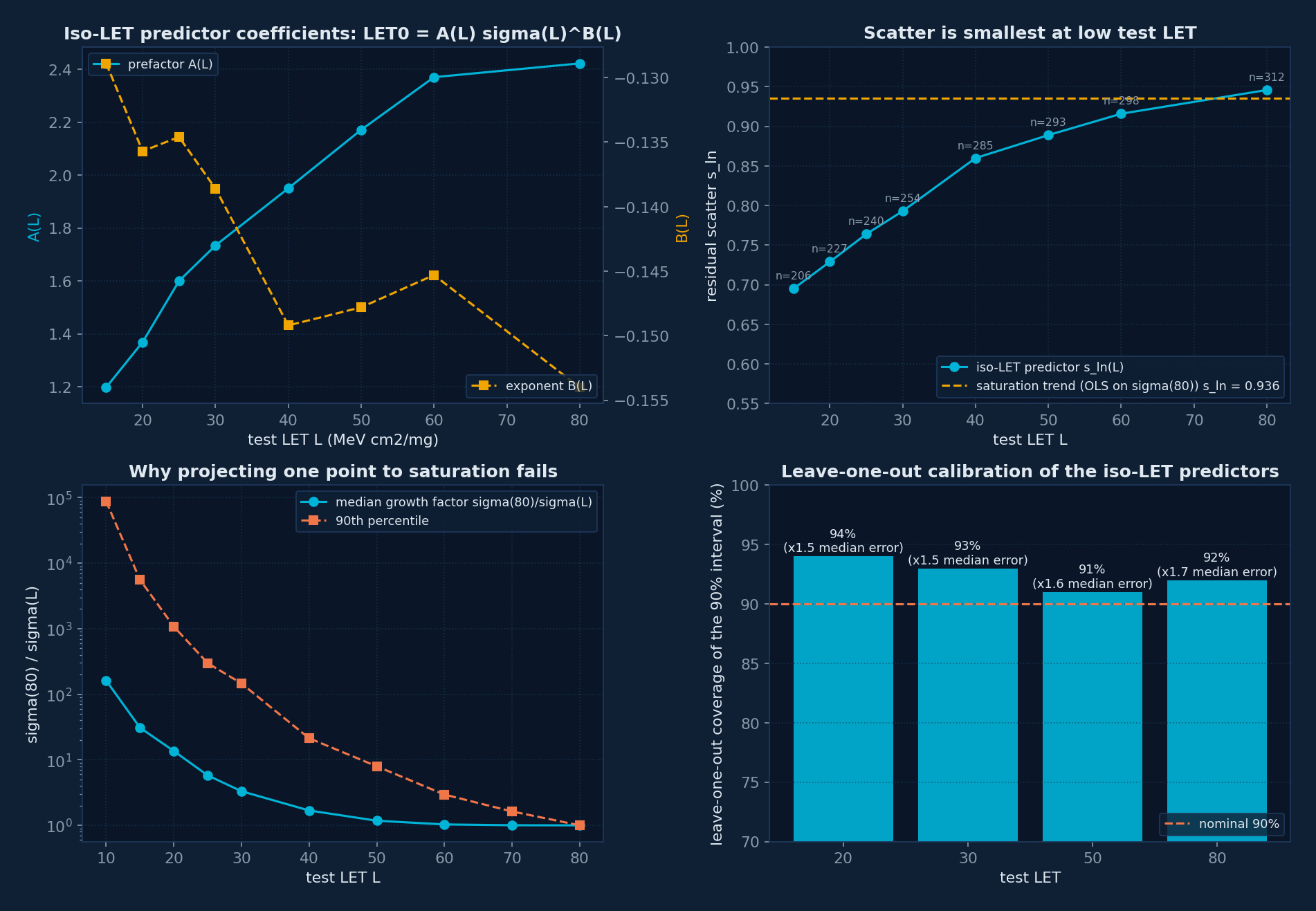
A designer who has one run at LET 20 or 30 with observed events cannot project σ to saturation: in the corpus the growth factor σ(80)/σ(20) has median x14 with a 90th percentile near x1078 (Table 8). Instead, onset is regressed directly against σ evaluated at the tested LET L, over the parts observable there (σ(L) at or above 10⁻⁸ cm²), giving a family of trends LET0 = A(L)·σ(L)B(L) indexed by the observation LET. The saturation trend of Section 4 is the L = 80 member of the family. Scatter is smallest at low test LET (sln = 0.695 at 15, 0.793 at 30) and grows to the saturation value at 80: observability of events at low LET conditions strongly on low onset, and the cross section near onset encodes the distance above it. Because regressor and regressand derive from the same fit, the relation was re-estimated using measured σ at real runs within 5 MeV·cm²/mg of L; the coefficients and scatter reproduce, so the effect is not a fitting artifact. The tool interpolates A, B and sln linearly in ln L between the tabulated members and clamps to the 15 to 80 range.
Table 8. Iso-LET predictors (global) and corpus growth factors
| Test LET L | n | A(L) | B(L) | R² | sln(L) | median σ(80)/σ(L) | 90th percentile |
|---|---|---|---|---|---|---|---|
| 15 | 206 | 1.198 | -0.1289 | 0.288 | 0.695 | x31 | x5584 |
| 20 | 227 | 1.369 | -0.1357 | 0.285 | 0.729 | x14 | x1078 |
| 25 | 240 | 1.600 | -0.1346 | 0.270 | 0.764 | x5.79 | x299 |
| 30 | 254 | 1.734 | -0.1386 | 0.281 | 0.793 | x3.31 | x146 |
| 40 | 285 | 1.950 | -0.1492 | 0.293 | 0.860 | x1.69 | x21 |
| 50 | 293 | 2.171 | -0.1478 | 0.280 | 0.889 | x1.18 | x8 |
| 60 | 298 | 2.370 | -0.1453 | 0.262 | 0.916 | x1.03 | x3 |
| 80 | 312 | 2.422 | -0.1540 | 0.293 | 0.946 | x1.00 | x1 |
Calibration and sanity battery
Leave-one-out validation predicts each part's threshold from a model trained without it. The nominal 90% intervals cover 94%, 93%, 91% and 92% of parts at test LET 20, 30, 50 and 80, with median error factors of x1.5 to x1.7 (Table 9). An external check applies the L = 30 predictor to CERN parts with full Weibull curves and covers 94% of the CERN onsets with a median error factor of 1.7 and a bias of +0.13 in ln units: the model under-predicts CERN onsets by about 13%, consistent with the CERN L0 being the Weibull onset parameter rather than the 10⁻⁸ crossing. Eight sanity checks were run on the final data: a fit-pathology census (18% of fits onset-pinned; 32 fitted asymptotes above 0.5 cm², excluded from σ(80) use by the measured-range flag where applicable), the σ(80) validation of Section 3, the circularity check above, leave-one-out coverage, bootstrap uncertainty, a one-entry-per-part duplicate test, heteroscedasticity by decade, and the external CERN check.
Table 9. Leave-one-out calibration of the iso-LET predictors
| Test LET | coverage of the 90% interval | median error factor |
|---|---|---|
| 20 | 94% | x1.5 |
| 30 | 93% | x1.5 |
| 50 | 91% | x1.6 |
| 80 | 92% | x1.7 |
11. Temperature
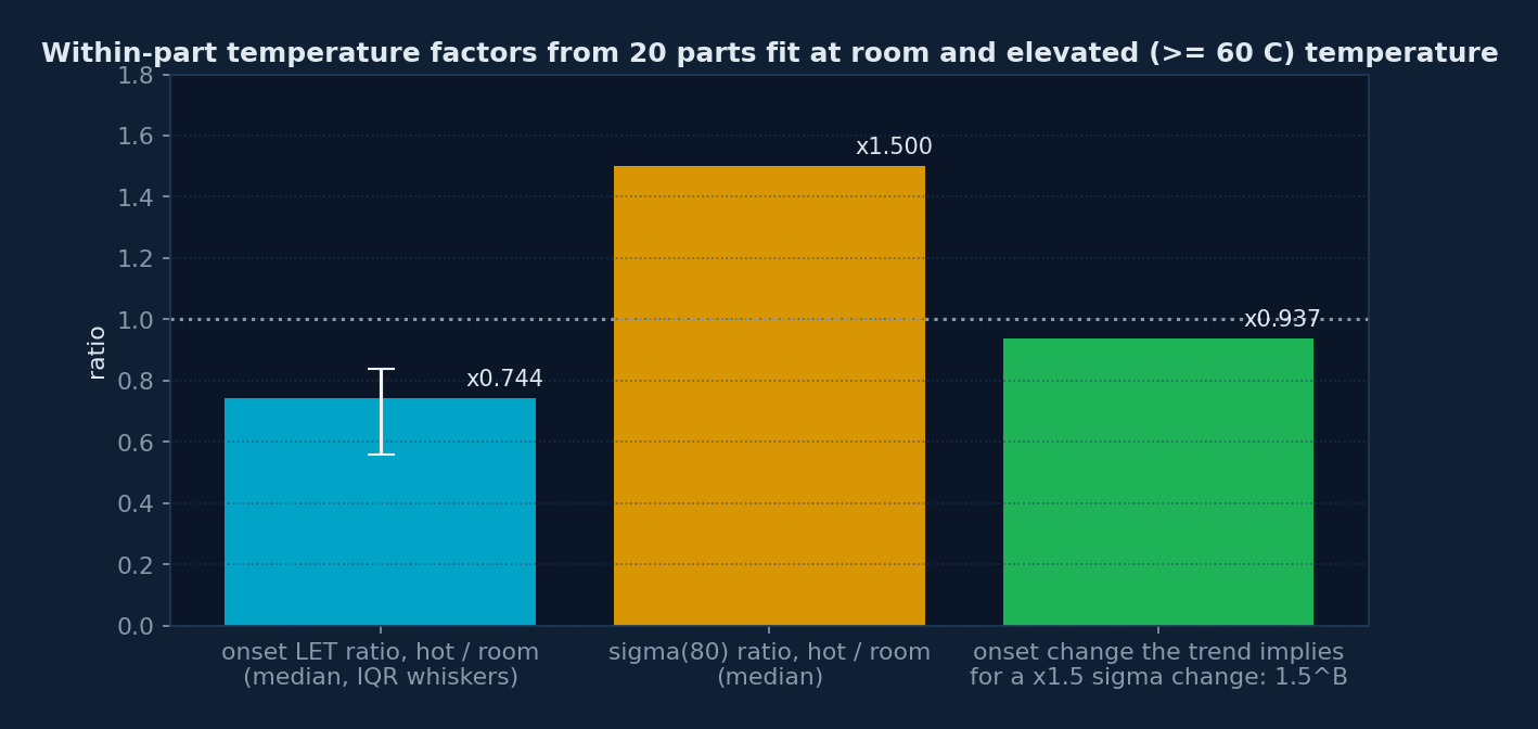
20 parts were fit at both room and elevated (at or above 60 °C) temperature. Within part, heating lowers the onset by a median factor 0.744 (interquartile range 0.56 to 0.84) and raises σ(80) by a median factor 1.5. A heated part therefore moves along the trend line: the slope predicts a factor 0.937 in onset for a factor 1.5 in σ, and the residual is about 20%. This is why the temperature covariate in the regression is null: given σ(80) measured hot, the trend already predicts the hot onset. The practical rule for translating room-temperature results is the within-part factor pair, which the tool exposes as a separate step (the elevated-temperature checkbox), and which the susceptibility priors use to map a room-temperature null at LET X to a hot-equivalent LET 0.74·X.
12. Mechanism screening
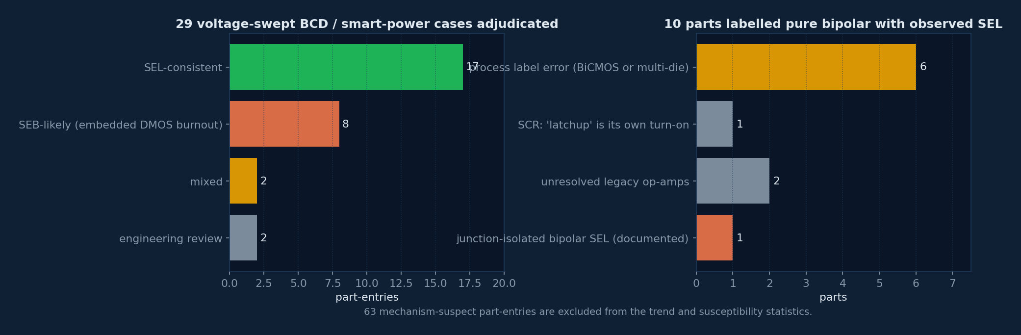
Three physics screens precede the statistics. Device screens: parts without pnpn structures (dielectrically isolated bipolar, GaN, SiC, discrete diodes and transistors, JFETs) cannot exhibit SEL, and observed events override the heuristic. SEL versus embedded-DMOS burnout in BCD and smart-power parts: the discriminating signature, input voltage stepped at fixed LET, clean at low bias, destructive at 40 to 90% of rated voltage without recovery, was detected from per-run bias records in 29 voltage-swept cases and adjudicated against the report language: 17 SEL-consistent, 8 burnout-likely, 2 mixed and 2 held for engineering review. Temperature-enhanced failure voltage and the absence of an internal DMOS stage served as SEL-confirming counter-signatures. Bipolar contradictions: ten parts labeled pure bipolar with observed SEL resolved into six process-label errors (BiCMOS or multi-die), one SCR whose "latchup" is its own triggered turn-on, two unresolved legacy operational amplifiers, and one documented exception, junction-isolated bipolar latchup [5]. Sixty-three mechanism-suspect part-entries are excluded from the trend and susceptibility statistics.
13. Censoring-aware susceptibility priors
Ladbury-style probabilities of SEL susceptibility per technology bucket [3] were updated on 1,845 classified part-entries (all-eras stratum; 630 in the modern stratum) with a Beta prior of pseudo-count m = 4 centered on the expert prior of [3] and a likelihood that uses the censored majority as evidence:
clean to hot-equivalent LET Xeff at fluence F: L(p) = (1 − p) + p·[1 − w(Xeff, F)·Fb(Xeff)]
Xeff = X for tests at or above 60 °C, 0.74·X at room temperature; unstated fluence: F = 10⁶ ions/cm²
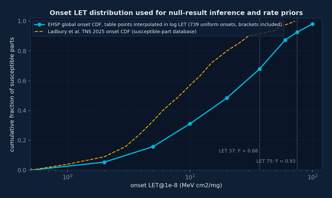
Here Fb is the bucket's onset CDF, shrunk toward the global onset CDF with k = 20 pseudo-observations, and w(X, F) is the censoring credit: the probability that a susceptible part with onset below X would have produced at least one event at fluence F, averaged over the corpus Weibull curves of 316 fitted susceptible parts. This replaces the fixed weights of earlier versions (1.0, 0.75, 0.5 for hot and high-fluence, high-fluence, and unstated-fluence tests), which were the dominant sensitivity of the previous model. For each censored part only the strongest statement, the highest credited LET, is kept. Posteriors are computed on a grid and summarized as a Beta(α, β) approximation, mean and 90% credible interval, so that downstream tools can sample them. The global onset CDF is built from 739 uniform onsets (fitted crossings and onset brackets, with the CERN onsets admitted to the CDF only) and is shipped in the model file (Figure 14).
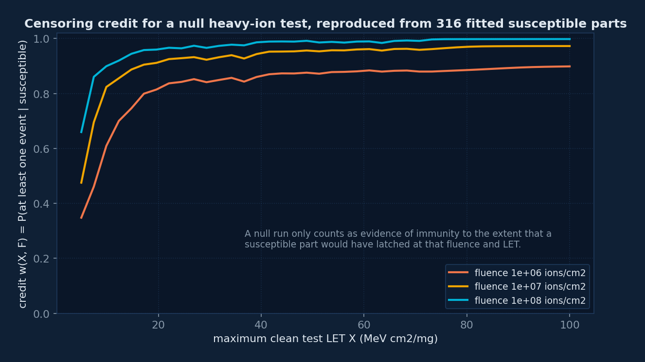
Table 10. Censoring credit at two clean-LET values
| fluence (ions/cm²) | w at X = 75 | w at X = 100 |
|---|---|---|
| 1e6 | 0.882 | 0.899 |
| 1e7 | 0.965 | 0.973 |
| 1e8 | 0.998 | 0.998 |
Strata
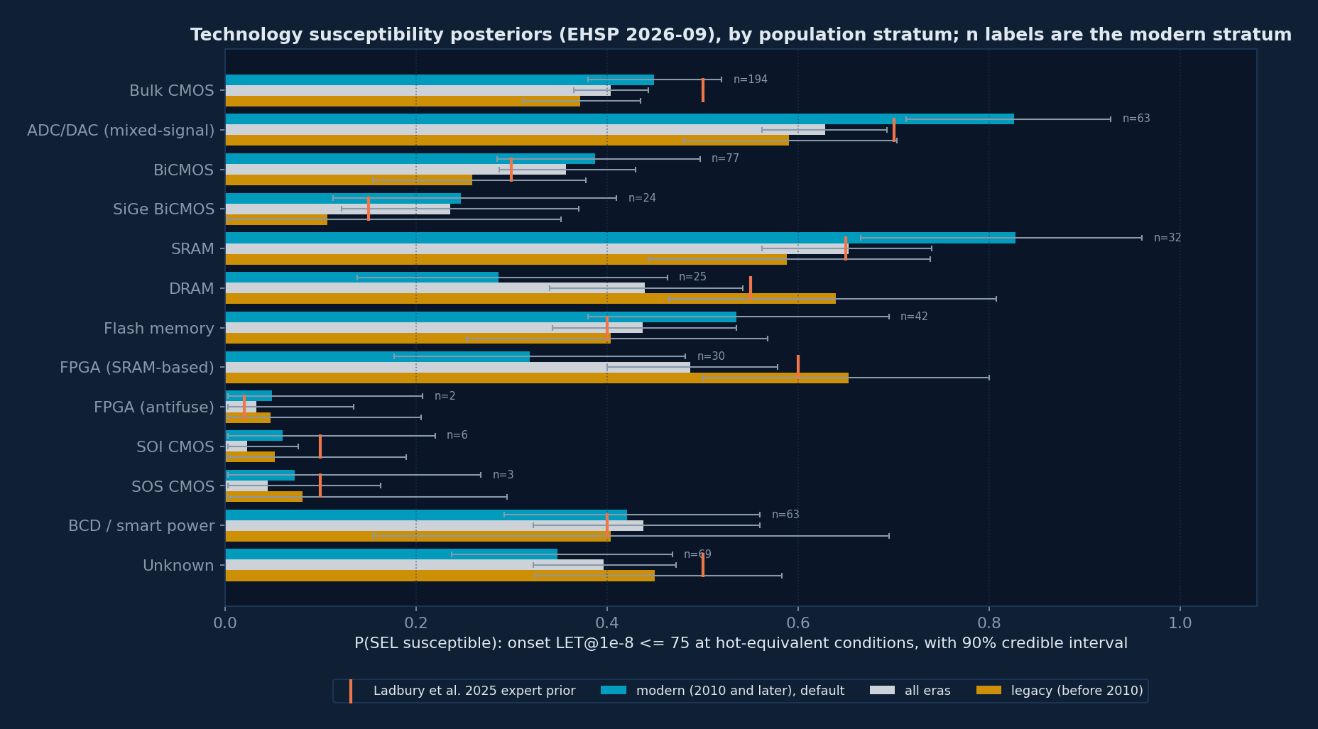
Priors are population-dependent, so the model carries every bucket in nine strata: by era (modern, all, legacy) and by source population (papers only; compendia, meaning the REDW data workshop and NASA GSFC summaries; proprietary test reports; mission-candidate parts, meaning compendia plus test reports, in all eras and modern only; and the customer-selected COTS parts of recent Space-RHA campaigns). The modern stratum is the default for designers. The Space-RHA campaign stratum differs most for BiCMOS (0.64 against 0.39 in the modern stratum) and SiGe (0.48 against 0.25, on very few parts), and is slightly higher for bulk CMOS (0.47 against 0.45); the difference is a selection effect, since parts reach those campaigns because a customer already suspected them.
Table 11. Part-entries per stratum
| Stratum | part-entries | with observed onset at or below 75 | raw fraction |
|---|---|---|---|
| all eras | 1,845 | 610 | 0.33 |
| modern (2010 and later), default | 630 | 216 | 0.34 |
| legacy (before 2010) | 568 | 194 | 0.34 |
| conference and journal papers only | 991 | 320 | 0.32 |
| compendia (REDW data workshop and NASA GSFC summaries) | 697 | 217 | 0.31 |
| proprietary test reports | 411 | 152 | 0.37 |
| mission-candidate parts (compendia + test reports) | 1,080 | 362 | 0.34 |
| modern mission-candidate parts | 444 | 156 | 0.35 |
| Space-RHA campaigns 2022-26 (customer-selected COTS) | 111 | 45 | 0.41 |
Table 12. Posterior P(SEL-susceptible), mean [90% credible interval], by bucket and stratum
| Bucket | Ladbury prior [3] | modern (2010 and later), default | all eras | legacy (before 2010) | modern mission-candidate parts | Space-RHA campaigns 2022-26 (customer-selected COTS) |
|---|---|---|---|---|---|---|
| Bulk CMOS | 0.50 | 0.45 [0.38, 0.52] n = 194, 69 susceptible | 0.40 [0.36, 0.44] n = 609, 195 susceptible | 0.37 [0.31, 0.43] n = 197, 63 susceptible | 0.46 [0.38, 0.54] n = 153, 55 susceptible | 0.47 [0.31, 0.65] n = 33, 11 susceptible |
| ADC/DAC (mixed-signal) | 0.70 | 0.83 [0.71, 0.93] n = 63, 40 susceptible | 0.63 [0.56, 0.69] n = 215, 111 susceptible | 0.59 [0.48, 0.70] n = 75, 35 susceptible | 0.90 [0.79, 0.98] n = 46, 32 susceptible | 0.85 [0.62, 0.98] n = 8, 6 susceptible |
| BiCMOS | 0.30 | 0.39 [0.28, 0.50] n = 77, 23 susceptible | 0.36 [0.29, 0.43] n = 197, 48 susceptible | 0.26 [0.15, 0.38] n = 49, 10 susceptible | 0.42 [0.30, 0.55] n = 57, 19 susceptible | 0.64 [0.44, 0.83] n = 20, 11 susceptible |
| SiGe BiCMOS | 0.15 | 0.25 [0.11, 0.41] n = 24, 5 susceptible | 0.24 [0.12, 0.37] n = 36, 7 susceptible | 0.11 [0.00, 0.35] n = 3, 0 susceptible | 0.23 [0.08, 0.42] n = 16, 3 susceptible | 0.48 [0.20, 0.77] n = 4, 3 susceptible |
| SRAM | 0.65 | 0.83 [0.67, 0.96] n = 32, 20 susceptible | 0.65 [0.56, 0.74] n = 130, 65 susceptible | 0.59 [0.44, 0.74] n = 48, 20 susceptible | 0.71 [0.46, 0.93] n = 11, 6 susceptible | 0.72 [0.37, 0.96] n = 1, 1 susceptible |
| DRAM | 0.55 | 0.29 [0.14, 0.46] n = 25, 4 susceptible | 0.44 [0.34, 0.54] n = 107, 31 susceptible | 0.64 [0.47, 0.81] n = 33, 15 susceptible | 0.30 [0.14, 0.51] n = 20, 3 susceptible | none |
| Flash memory | 0.40 | 0.54 [0.38, 0.69] n = 42, 16 susceptible | 0.44 [0.34, 0.54] n = 115, 35 susceptible | 0.40 [0.25, 0.57] n = 33, 10 susceptible | 0.43 [0.28, 0.61] n = 31, 10 susceptible | 0.42 [0.13, 0.76] n = 4, 1 susceptible |
| FPGA (SRAM-based) | 0.60 | 0.32 [0.18, 0.48] n = 30, 6 susceptible | 0.49 [0.40, 0.58] n = 114, 44 susceptible | 0.65 [0.50, 0.80] n = 35, 19 susceptible | 0.46 [0.24, 0.71] n = 16, 4 susceptible | none |
| FPGA (antifuse) | 0.02 | 0.05 [0.00, 0.21] n = 2, 0 susceptible | 0.03 [0.00, 0.14] n = 6, 0 susceptible | 0.05 [0.00, 0.20] n = 2, 0 susceptible | 0.05 [0.00, 0.21] n = 2, 0 susceptible | none |
| SOI CMOS | 0.10 | 0.06 [0.00, 0.22] n = 6, 0 susceptible | 0.02 [0.00, 0.08] n = 26, 0 susceptible | 0.05 [0.00, 0.19] n = 7, 0 susceptible | 0.10 [0.00, 0.35] n = 2, 0 susceptible | 0.10 [0.00, 0.37] n = 1, 0 susceptible |
| SOS CMOS | 0.10 | 0.07 [0.00, 0.27] n = 3, 0 susceptible | 0.04 [0.00, 0.16] n = 8, 0 susceptible | 0.08 [0.00, 0.29] n = 2, 0 susceptible | 0.10 [0.00, 0.35] n = 1, 0 susceptible | none |
| BCD / smart power | 0.40 | 0.42 [0.29, 0.56] n = 63, 17 susceptible | 0.44 [0.32, 0.56] n = 80, 23 susceptible | 0.40 [0.15, 0.69] n = 7, 2 susceptible | 0.43 [0.29, 0.58] n = 52, 14 susceptible | 0.43 [0.26, 0.63] n = 29, 8 susceptible |
| Unknown | 0.50 | 0.35 [0.24, 0.47] n = 69, 16 susceptible | 0.40 [0.32, 0.47] n = 202, 51 susceptible | 0.45 [0.33, 0.58] n = 77, 20 susceptible | 0.42 [0.27, 0.59] n = 37, 10 susceptible | 0.50 [0.26, 0.76] n = 11, 4 susceptible |
Sensitivities
Prior strength m is negligible for buckets with n above 100. Moving the susceptibility cutoff to 60 or 100 changes posteriors by about 0.03 (BiCMOS 0.05). Restricting to parts whose process label carries high confidence lowers bulk CMOS, flash and BCD by 0.05 to 0.09, a systematic effect of label pollution in the other direction. The fixed censoring weights of the previous model were worth 0.15 and are gone.
14. Validation of the priors
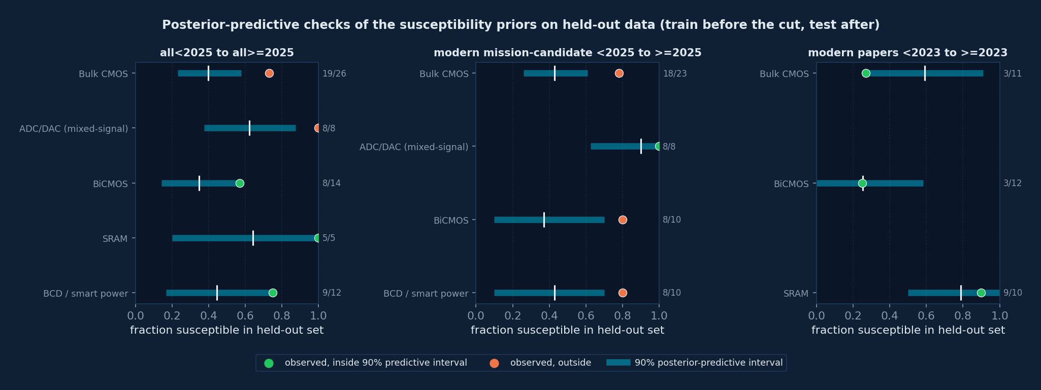
The priors were checked by posterior-predictive tests on held-out data: train on parts before a cut year, predict the number of susceptible parts among held-out parts with a decisive outcome (onset at or below 75, or clean to at least LET 55 with credit at least 0.8), and ask whether the observed count falls inside the 90% Beta-binomial predictive interval (Table 13, Figure 15). On held-out modern papers (train before 2023, test 2023 and later) every bucket is inside. On the 2025-26 holdouts, which are dominated by recent proprietary campaigns, bulk CMOS, converters, BiCMOS and BCD parts exceed the literature-trained predictions in one or both splits: the parts that reach a commercial test campaign in 2025 are selected toward risk. That failure is the reason the model carries a dedicated Space-RHA campaign stratum rather than a single population prior, and it is why the tool lets the user choose the stratum.
Table 13. Posterior-predictive checks
| Split (train to test) | Bucket | held-out n | observed susceptible | fraction | predicted mean | 90% predictive count | result |
|---|---|---|---|---|---|---|---|
| all<2025 to all>=2025 | Bulk CMOS | 26 | 19 | 0.73 | 0.40 | [6, 15] | outside |
| all<2025 to all>=2025 | ADC/DAC (mixed-signal) | 8 | 8 | 1.00 | 0.62 | [3, 7] | outside |
| all<2025 to all>=2025 | BiCMOS | 14 | 8 | 0.57 | 0.35 | [2, 8] | inside |
| all<2025 to all>=2025 | SRAM | 5 | 5 | 1.00 | 0.64 | [1, 5] | inside |
| all<2025 to all>=2025 | BCD / smart power | 12 | 9 | 0.75 | 0.44 | [2, 9] | inside |
| modern mission-candidate <2025 to >=2025 | Bulk CMOS | 23 | 18 | 0.78 | 0.43 | [6, 14] | outside |
| modern mission-candidate <2025 to >=2025 | ADC/DAC (mixed-signal) | 8 | 8 | 1.00 | 0.90 | [5, 8] | inside |
| modern mission-candidate <2025 to >=2025 | BiCMOS | 10 | 8 | 0.80 | 0.37 | [1, 7] | outside |
| modern mission-candidate <2025 to >=2025 | BCD / smart power | 10 | 8 | 0.80 | 0.43 | [1, 7] | outside |
| modern papers <2023 to >=2023 | Bulk CMOS | 11 | 3 | 0.27 | 0.59 | [3, 10] | inside |
| modern papers <2023 to >=2023 | BiCMOS | 12 | 3 | 0.25 | 0.25 | [0, 7] | inside |
| modern papers <2023 to >=2023 | SRAM | 10 | 9 | 0.90 | 0.79 | [5, 10] | inside |
15. How the tool uses the model
All four input modes call the same SelModel API that ships with the model file; the numbers shown as "EHSP API"
in the result tiles are its direct output, and the 14 test vectors embedded in the file are run against it
by selftest(). The Monte Carlo layers add the Poisson uncertainty of a measured cross section and the hard
constraints that a latching test imposes.
SEL observed at the test LET (events and fluence, or cross section)
The iso-LET member at the test LET is used (Section 10). With n events at fluence F the cross section is drawn from a Gamma(n + 1/2)/F posterior (Jeffreys prior on the Poisson rate); with a cross section given directly it is fixed. Each of 20,000 draws gives ln LET0 = ln A(L) + B(L)·ln σ + sln(L)·z. Draws at or above the test LET are discarded: a part that latched at L has its 10⁻⁸ crossing below L, a hard constraint that the regression alone does not know. Median and quantiles are reported from the surviving draws, with the fraction removed shown as a diagnostic; when more than half of the trend mass sits above the test LET the measurement is onset-dominated and the tool says so. The cross-check line reports what the saturation trend and the CERN trend would have given had the cross section been treated as saturated, together with the corpus growth factor at that LET (Table 8), which is why that assumption is not made. For SRAM the density-gated prior of Section 9 replaces the regression, truncated in the same way.
Saturated cross section
predictOnset({sigma_sat, device_class, era}) selects the partially pooled class trend for the chosen era
when the group has at least eight entries and the global errors-in-variables trend otherwise, and returns the median and the
scatter; the tool converts the scatter to the requested confidence level, truncates at LET 80 (a measured σ(80) implies
the part latched there), and reports the global, OLS and CERN values alongside. Classes that carry a prior but no trend (SiGe,
SOI, SOS, antifuse) use the global trend.
Temperature
With the elevated-temperature box unchecked, the tool reports the as-tested (room) result and a hot-equivalent median scaled
by 0.744. With it checked in the saturated mode, the room-temperature trend prediction is scaled by
0.744 and the interval bounds by the interquartile factors [0.56,
0.84], exactly as predictOnset({hot: true}) does. In the null mode the checkbox
sets Xeff.
Null result
The null branch applies the construction of Section 13 to one part. The prior P(susceptible) is the bucket's posterior in the chosen stratum. Candidate onsets for a susceptible part are drawn from the global onset CDF conditioned on onset at or below 75, interpolated in ln LET between the tabulated points. A candidate above Xeff is untouched by the data (likelihood one). A candidate below it is weighted by the corpus probability of zero events, P(0 | onset bin, X, F), tabulated from the same 316 susceptible Weibull curves on a grid of onset bins, test LETs from 5 to 100 and fluences from 10⁵ to 10⁹, smoothed to be non-decreasing in onset (Table 14, file embedded in this page) and interpolated linearly in X and in ln F. The average likelihood over candidates is the part-specific P(null | susceptible), so the posterior probability of susceptibility is p·P(null | susceptible) / [p·P(null | susceptible) + (1 − p)], and the weighted candidates give the threshold posterior for the case that the part is susceptible after all. This follows the logic of Ladbury, Joplin and Lauenstein [6] for bounding rates from null results, with the corpus curves replacing an assumed conditional cross-section distribution. Raising the fluence tightens the exclusion of low onsets; nothing about the test probes above Xeff.
Table 14. P(zero events | susceptible part with onset in bin, test at LET X), fluence 10⁷ ions/cm²
| test LET X | 0.5 to 1 | 1 to 2 | 2 to 3 | 3 to 5 | 5 to 7.5 | 7.5 to 10 | 10 to 15 | 15 to 20 | 20 to 30 | 30 to 40 | 40 to 50 | 50 to 60 | 60 to 75 |
|---|---|---|---|---|---|---|---|---|---|---|---|---|---|
| 20 | 0.000 | 0.000 | 0.004 | 0.004 | 0.007 | 0.007 | 0.047 | 0.323 | |||||
| 40 | 0.000 | 0.000 | 0.003 | 0.003 | 0.007 | 0.007 | 0.013 | 0.033 | 0.122 | 0.216 | |||
| 60 | 0.000 | 0.000 | 0.003 | 0.003 | 0.007 | 0.007 | 0.013 | 0.033 | 0.074 | 0.074 | 0.125 | 0.125 | |
| 75 | 0.000 | 0.000 | 0.003 | 0.003 | 0.007 | 0.007 | 0.013 | 0.033 | 0.070 | 0.070 | 0.100 | 0.100 | 0.258 |
Empty cells are bins with fewer than three corpus parts below X; the tool walks down to the nearest populated bin. The other SEL tools on this site consume the same file: the SEL Test-LET Tool takes the modern susceptibility posteriors for its technology mix and the global onset CDF as its default prior (interpolating that CDF linearly in LET, as the paper it implements does); the SEE Rate Assessment Tool takes the modern posteriors as its bounding priors and the global errors-in-variables trend for untested parts; and the SEE Cross-Section Tool offers the global and class trends for its single-point method.
16. Limitations
Extrapolated thresholds (63% of the trend set) depend on fitted shape and should be floored at the lowest tested LET for conservative use. Per-part uncertainties come from a parametric bootstrap that conditions on the fitted model, so they understate uncertainty for parts whose fits sit at parameter bounds. Interval censoring assumes the true 10⁻⁸ crossing lies between the fitted crossing, less one standard error, and the lowest tested LET; a fully Bayesian per-part posterior would remove that assumption. Bias voltage is not a covariate. Per-device cross sections conflate die area; a die-area normalization would likely resolve the high-σ excess and is the principal remaining refinement. The iso-LET predictors remain ordinary regressions on fitted inputs, justified by their leave-one-out calibration rather than by a measurement-error model. The class trends are thin for several groups and the legacy-era groups are thinner still. The susceptibility priors depend on process labels whose confidence varies, and the held-out 2025-26 checks show that a literature-trained prior under-predicts the risk of parts selected for commercial campaigns; the stratum selector exists for that reason and no single number should be quoted without its stratum. The mechanism screen depends on per-run bias records that reports before about 2000 lack. Onset in this model is a fitted 10⁻⁸ crossing under the tested conditions; it is not a guarantee of immunity below it, and the SEL Test-LET tool should be used for system-level screening decisions.
17. Reproducibility and files
The site publishes one file for this model, ehsp-2026-09.js (release 2026-09,
built 2026-09-02), which carries the fitted parameters and the SelModel API. The null-result
likelihood table is embedded in this page, and the numbers printed in this section are baked in at build time.
No source data files are published.
The figures and tables are generated by build_methodology_figs.py and build_methodology_html.py from the
model file and the internal fit set, which plots proprietary entries only as anonymous points. Internally, the pipeline is
fit_sel_weibull.py (fits and tiers), boot_parts.py (per-part bootstrap), eiv_trend.py (the
errors-in-variables model and partial pooling), s80_iso.py (saturation and iso-LET predictors),
ladbury_update_v3.py (priors, strata and validation) and priors_sensitivity.py; all are designed to
be rerun as the corpus grows. The full-corpus fit set and the per-part data are not published because a large part of the
corpus is proprietary; the published subset is available in aggregate on the
REDW distributions page.
To verify the tool against the model file in a browser console: SelModel(EHSP_MODEL).selftest() prints the
number of mismatched test vectors, which should be zero.
18. References
[1] R. Ladbury, "Under-Constrained SEE Data: Implications for Estimating and Bounding SEE Rates," IEEE Trans. Nucl. Sci., vol. 71, no. 4, pp. 680-689, Apr. 2024 (presented at NSREC 2023). The Poisson-likelihood fitting framework, the Bayesian use of an onset versus cross-section prior, and the CERN-database trend.
[2] A. Coronetti and R. García Alía, CERN single-event latchup database, published as Table II of [1]; the 51-part curated subset defines the CERN 2023 trend LET0 = 1.9638 σs−0.192, sln = 0.82.
[3] R. Ladbury, G. R. Allen, F. Irom, R. Gaza, S. Vartanian, J. D. Barth and R. F. Hodson, "Statistical Analysis of Historical SEL Test Data to Provide a Priori Risk Estimates for Use of Unhardened CMOS Parts," IEEE Trans. Nucl. Sci., vol. 72, no. 4, pp. 1094-1101, Apr. 2025. The technology susceptibility priors and the 66-part onset-LET distribution.
[4] T. E. Page and J. M. Benedetto, "Extreme Latchup Susceptibility in Modern Commercial-off-the-Shelf (COTS) Monolithic 1M and 4M CMOS Static Random-Access Memory (SRAM) Devices," IEEE Radiation Effects Data Workshop, 2005. SEL at the lowest available LET in high-density COTS SRAM.
[5] M. Shoga, R. Gorelick, R. Rau, R. Koga and S. Martinez, "Observation of Single Event Latchup in Bipolar Devices," IEEE Radiation Effects Data Workshop, 1993. The documented junction-isolated bipolar latchup exception.
[6] R. Ladbury, M. Joplin and J.-M. Lauenstein, "Bounding SEL Rates for Null Results and Other Limited Test Data," IEEE Trans. Nucl. Sci., 2026, DOI 10.1109/TNS.2026.3662106. Null-result bounding logic.
[7] R. DerSimonian and N. Laird, "Meta-analysis in clinical trials," Controlled Clinical Trials, vol. 7, no. 3, pp. 177-188, 1986. The random-effects shrinkage used for partial pooling of class trends.
[8] R. Ladbury and M. Joplin, "System-Level Risk Assessment for Single-Event Latchup (SEL) Based on Historical Data," IEEE Trans. Nucl. Sci., 2026, DOI 10.1109/TNS.2026.3706172. The system-level screening method implemented by the SEL Test-LET Tool, which consumes this model's priors and onset CDF.
[9] IEEE Radiation Effects Data Workshop records, 1992 to 2025, and RADECS data-workshop records; RADECS Proceedings and IEEE Trans. Nucl. Sci., 1991 to 2025; NASA Goddard Space Flight Center radiation effects and analysis test reports and compendia. Public sources of the corpus, re-extracted from the primary documents.
[10] Proprietary heavy-ion test reports and structured campaign records. Used in aggregate for the fits, trends and priors of this model; not available for public citation and not shown individually anywhere on this site.
[11] G. R. Allen, uniform reanalysis of single-event latchup onset and saturation across the combined SEL test corpus, manuscript in preparation, 2026; Extended Historical SEL Priors (EHSP), release 2026-09, Space-RHA (this page and the model file).